Your first design#

This tutorial builds a complete, ready-to-run experimental design from scratch. At the end you will have a table of 30 experiment coordinates saved as a CSV file, and you will know what every line of code did.

No prior knowledge of design of experiments is assumed.

The problem#

Suppose you study a chemical process with three inputs you can control: a temperature between 300 and 500 K, a pressure between 1 and 5 bar, and a catalyst loading that your lab stocks in four fixed concentrations. You can afford 30 experimental runs. Which 30 combinations of the three inputs should you run?

Picking combinations by hand, or on a regular grid, wastes runs: points cluster, whole regions stay unexplored, and two inputs often end up correlated by accident. A space-filling design spreads the runs so that every region of the input space is represented. That is what Mergen computes.

Step 1: define the parameter space#

import mergen

space = mergen.ParameterSpace({
    'temperature': ('continuous', 300, 500),
    'pressure':    ('continuous', 1.0, 5.0),
    'catalyst':    [0.1, 0.2, 0.5, 1.0],
})

Each key is a parameter name, each value describes what the parameter can take. A ('continuous', low, high) tuple declares a continuous range. A plain list declares a discrete parameter: only these exact values will ever appear in the design, which matches how a stock of fixed catalyst concentrations behaves in the lab.

Other parameter types (integer, logarithmic, nominal, ordinal) are covered in the how-to guides.

Step 2: create a sampler and set the budget#

sampler = mergen.Sampler(space)
sampler.set_design(n_samples=30)

The sampler owns the design process. n_samples is your experimental budget. Thirty runs for three parameters follows the common 10 runs per dimension guideline for computer experiments (Loeppky, Sacks & Welch, 2009); the choosing-a-sample-size page in the explanation section discusses when to deviate from it.

Step 3: run the optimisation#

result = sampler.run(criteria='umaxpro', algorithm='sa', seed=44)

Mergen starts from a Latin hypercube arrangement and iteratively improves it: the uMaxPro criterion scores how well the points fill the space, and the sa (simulated annealing) optimiser searches for the arrangement with the best score. Progress is printed as it runs; expect on the order of a minute for a design of this size.

Passing a seed makes the run reproducible. The defaults used here are sensible general-purpose choices; which criterion and optimiser to prefer for a given problem is exactly what the explanation section is for.

Step 4: look at the result#

print(result.samples.head())

    temperature  pressure  catalyst point_type
id
0    417.171717  2.979798       0.5  Optimised
1    304.040404  1.686869       0.1  Optimised
2    491.919192  4.191919       0.2  Optimised
...

result.samples is a pandas DataFrame with one row per experimental run. The point_type column records how each row entered the design; in this tutorial every point is Optimised, but designs can also contain prescribed points and focus-region points (see the how-to guides).

You may notice the run banner also reported a small validation set. Mergen sets aside additional space-filling points (by default 20 % of n_samples, accessible as result.validation) that are maximally far from the design points. If you later fit a surrogate model to your results, these are honest test locations; if you do not need them, set n_validation=0 in set_design.

A quick visual check of what those 30 rows look like:

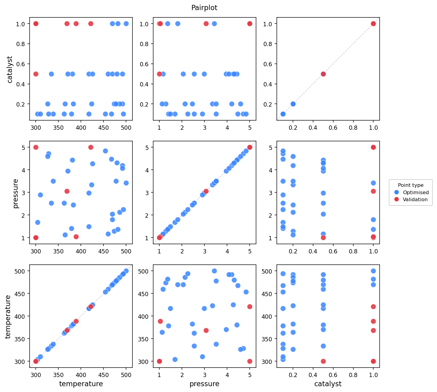
Pairwise scatter plots of the 30-run tutorial design. — The tutorial design (seed 44) in all pairwise projections. Points spread evenly, and the four catalyst levels form fully used bands.#

Step 5: export and run your experiments#

result.to_csv()

This writes the design table to the output directory reported in the console. Excel, LaTeX, HTML, JSON, and Markdown exports work the same way (to_excel(), to_latex(), and so on).

That is the complete workflow: define the space, set the budget, run, export. Five statements from an empty file to a defensible experimental plan.

Where to go next#

The next tutorial, understanding the output, teaches you to read the quality report and the diagnostic plots, so you can judge, and defend in writing, how good this design actually is.

References#

Loeppky, J. L., Sacks, J., & Welch, W. J. (2009). Choosing the sample size of a computer experiment: A practical guide. Technometrics, 51(4), 366-376.