Understanding the output

The previous tutorial produced a design. This one teaches you to judge it. Mergen’s position is that a design you cannot defend with numbers is not finished, so every result carries a quality report and diagnostic plots. This page walks through both.

We continue from the result object of the first tutorial:

result = sampler.run(criteria='umaxpro', algorithm='sa', seed=44)

The quality report

result.quality_report()

════════════════════════════════════════════════════════════════════
  MERGEN Design Metrics  (n=30, d=3)
════════════════════════════════════════════════════════════════════
  Metric                      Value    Baseline  Better when    Rank
────────────────────────────────────────────────────────────────────
  Min distance               0.0857      0.0505  higher      90th pct
  Minimax distance           0.7013      0.5851  lower        6th pct *
  Max |correlation|          0.3978      0.2386  lower        8th pct *
  2D projection CD2          0.2488      0.1890  lower        6th pct *
  CV distances               0.3908      0.4017  lower       72th pct
  Mean distance              0.7159      0.7415  higher      26th pct
────────────────────────────────────────────────────────────────────
  Criterion scores
────────────────────────────────────────────────────────────────────
  UMAXPRO                    8.7221e+15  1.2973e+22   100th pct  lower
────────────────────────────────────────────────────────────────────
  * = primarily optimised by 'umaxpro'
  Baseline: 300 MC designs from feasible space
════════════════════════════════════════════════════════════════════

Your numbers will differ in detail from run to run and from machine to machine; the structure is what matters.

The Monte Carlo baseline

Before printing, Mergen generates 300 random designs of the same size from the same feasible space and computes every metric for each of them. This baseline is what turns raw numbers into evidence. A minimum distance of 0.0857 means nothing in isolation; knowing that 300 random attempts averaged 0.0505 quantifies what the optimisation gained.

Reading a row

Each row has four parts.

Value is the metric computed on your design. Baseline is the mean of the same metric over the 300 random designs. Better when tells you the direction: for minimum distance, higher is better (points far from their nearest neighbour); for discrepancy-type metrics, lower is better.

Rank is direction-adjusted, so it always reads the same way: it is the share of baseline designs that your design beats on that metric. The 90th percentile min distance above outperforms 90 percent of the random designs; the 6th percentile minimax distance outperforms only 6 percent of them. Higher rank is always better, whatever the metric’s direction, and the terminal colour coding follows the same rule.

The asterisks

The rows marked * flag the metrics most closely related to the chosen criterion, as a guide to which rows deserve your attention first. The example above also illustrates an honest and important point: a design can sit at the 100th percentile on the criterion it optimised while ranking modestly on other classical metrics. A single criterion is one definition of a good design, not all of them. If the metrics you care about are not the ones your criterion serves, the fix is not more iterations but a different criterion; the choosing-a-criterion page in the explanation section maps goals to criteria, and mergen.compare() measures the trade-offs empirically.

The criterion row

The final block reports the optimised criterion itself against the same baseline. This is the single most direct statement of optimisation success. The 100th percentile here reads: no random design came anywhere near it. Note the scale: criterion values such as these are only meaningful relative to the baseline, never in absolute terms, which is why the report always prints both.

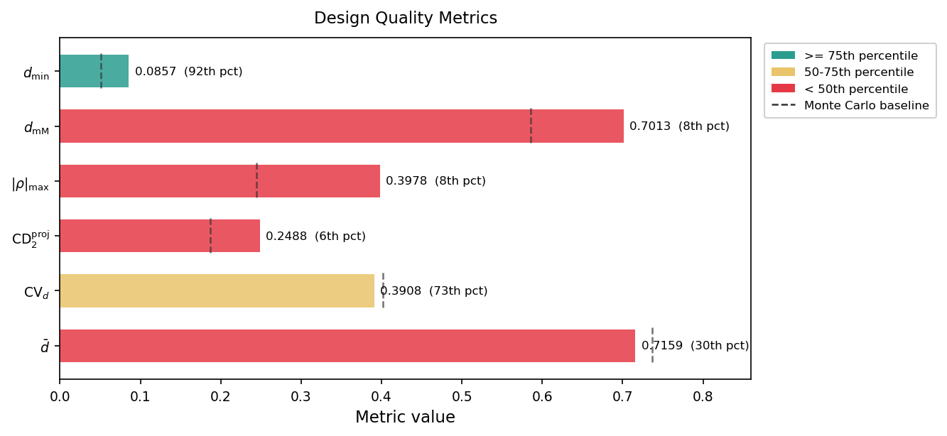
The same report as a chart: bar length is the metric value, the dashed line the Monte Carlo baseline, and colour encodes the percentile band. The mixed colours are the honest signature of a single-criterion optimisation, exactly as discussed above.

The diagnostic plots

result.plot('pairplot')

The pairplot draws every pairwise projection of the design. It is the fastest visual check for the two classic failure modes: clustering (two points nearly coincide in some projection, wasting a run) and holes (an empty region no run will ever probe). A healthy space-filling design looks evenly sprinkled in every panel, with the discrete catalyst values forming clean, fully used bands.

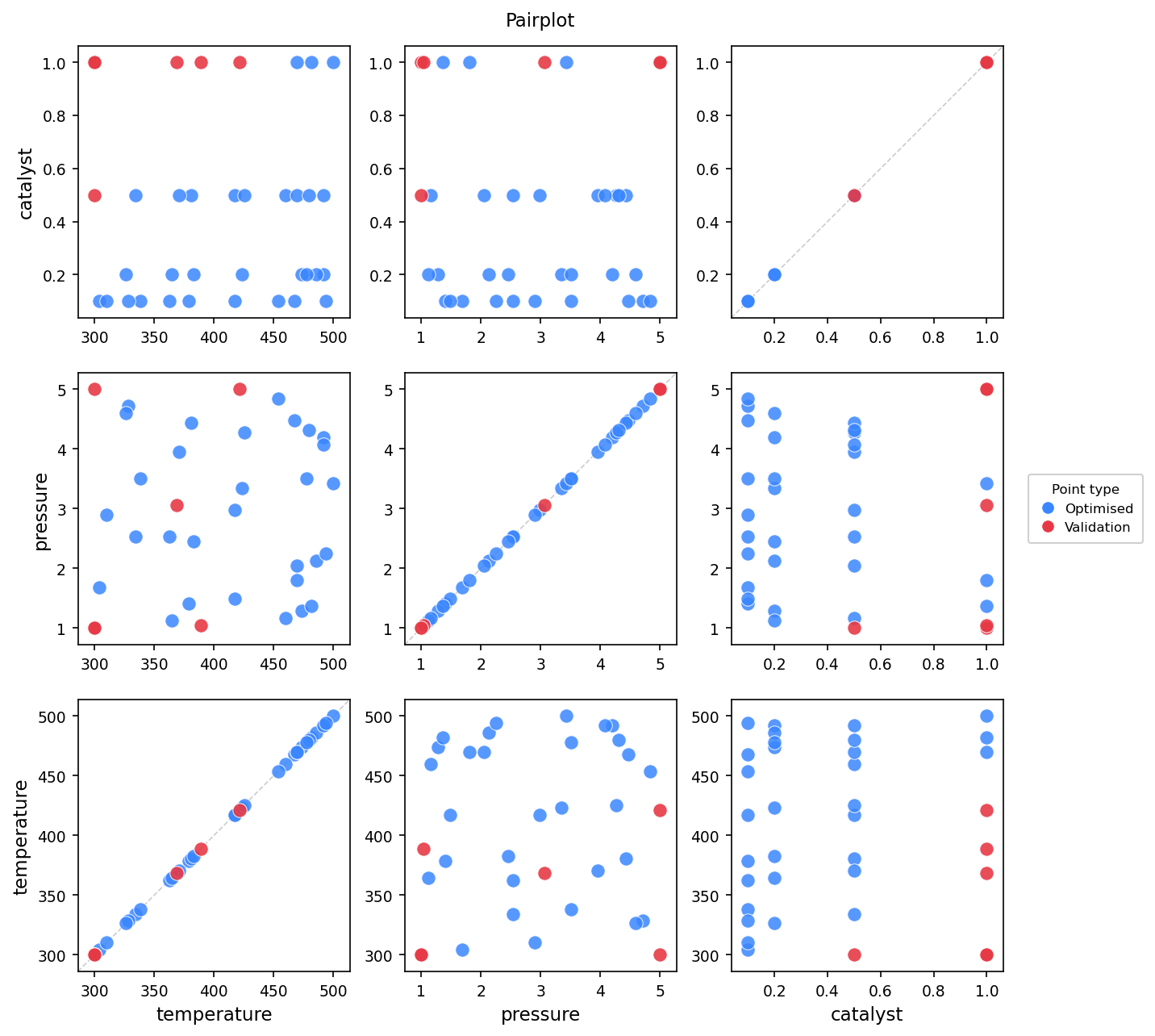
Every pairwise projection of the tutorial design. Validation points (reserved hold-out locations) are drawn in their own colour.

A complementary check is the one-dimensional view:

result.plot('1d')

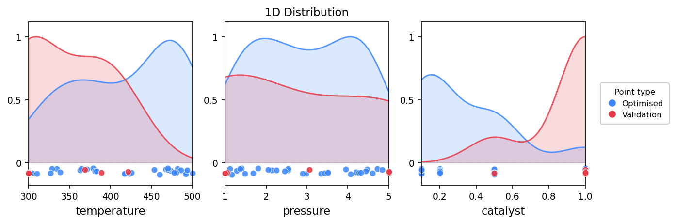
Marginal coverage per parameter: the strip shows the actual design values, the curve their smoothed density. Flat, band-free coverage in every panel is the Latin hypercube backbone doing its job.

result.plot('quality')

The quality plot, shown at the top of this page, renders the report graphically: each metric’s value against the Monte Carlo baseline, so a reviewer can see at a glance where the design sits relative to the random cloud.

Writing it up

For a paper’s methods section, the report gives you everything needed for a sentence of the form: “A 30-run space-filling design was generated with Mergen (criterion uMaxPro, simulated annealing); the design’s minimum inter-point distance ranked at the 90th percentile of 300 random reference designs.” Every number in that sentence comes from the table above, and result.to_latex() exports the design itself for the appendix.

Where to go next

If the report says the design is not good enough, do not tune blindly: read the choosing-a-criterion and choosing-an-optimiser pages in the explanation section, or let mergen.compare() sweep the combinations for you (covered in the how-to guides).