Choosing an optimiser

All three optimisers solve the same problem: given a criterion, search the space of grid-constrained Latin-hypercube designs for the arrangement with the best score. They share the move vocabulary (replacing or exchanging coordinates of design points on the candidate grid), respect all constraints and prescribed points, and are deterministic for a fixed seed. They differ in how they explore.

Simulated annealing ('sa')

Simulated annealing (Kirkpatrick, Gelatt & Vecchi, 1983) accepts improving moves always and worsening moves with probability \(\exp(-\Delta / T)\), where the temperature \(T\) decreases over the run. Early on, the search roams freely across the design space; as \(T\) falls, it settles into the best basin it has found. This is the classical defence against local optima, which space-filling landscapes have in abundance.

Mergen’s implementation removes the traditional tuning burden: the initial temperature is calibrated automatically by probing the energy landscape and solving for a target acceptance rate (following the approach of Ben-Ameur, 2004), and the run is repeated from independent starts (n_restarts, default 5) with the best result kept.

Use it as the default. It is the slowest of the three but the most robust across problem types, and its restart structure gives it the best chance on rugged landscapes such as heavily constrained spaces.

Stochastic coordinate exchange ('sce')

Stochastic coordinate exchange (Kang, 2019) iterates a simple, fast local search: pick a design point and a coordinate, try exchanging its value against candidate grid levels, keep the best. Without a temperature mechanism it commits to improvements immediately, which makes it markedly faster than annealing.

Use it when time matters and the problem is small to moderate, or as a quick first pass before committing to a long annealing run. On small problems its greediness costs little: in Mergen’s validation suite, sce attains the exhaustively verified global optimum on the one-dimensional test problems, as does sa.

Enhanced stochastic evolutionary ('ese')

The enhanced stochastic evolutionary algorithm (Jin, Chen & Sudjianto, 2005) also accepts some worsening moves, but controls acceptance with an adaptive threshold rather than a temperature schedule. Its distinguishing structural property is the move itself: ESE perturbs a design by swapping values between two rows within a single column. Such element exchanges preserve the set of levels used in every column exactly, so the marginal level histogram of the initial Latin hypercube survives the whole optimisation.

Use it when exact preservation of per-axis level frequencies is a requirement, for example when each level of a discrete factor must appear a fixed number of times.

One structural limitation follows directly from the move: with a single parameter (\(d = 1\)), swapping two values within the only column permutes the rows but leaves the design, as a set of points, unchanged, so ESE cannot improve any one-dimensional design. Sampler.run therefore raises an error for ese on one-parameter spaces and suggests sa or sce instead.

Practical guidance

Default to sa. Use sce when an answer is needed in seconds rather than minutes, or as the default optimiser inside large compare() sweeps. Use ese when marginal level balance must be preserved exactly and the space has at least two parameters.

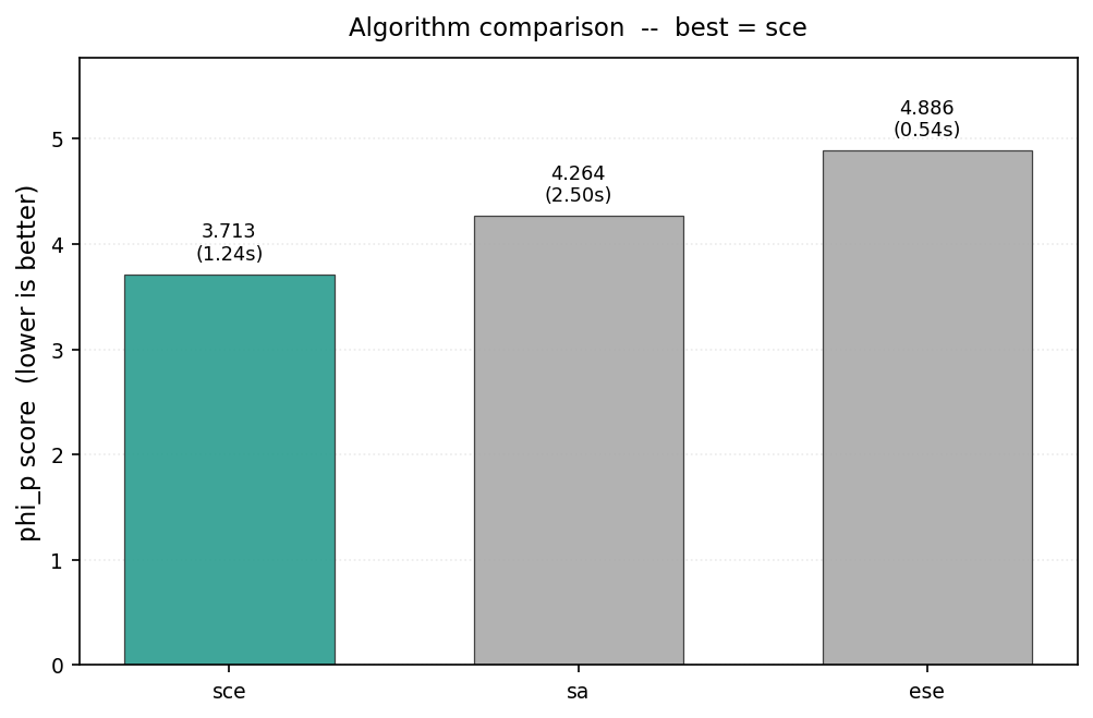
One criterion, three optimisers, one seeded problem: score (lower is better) with wall time annotated. Produced by sampler.run(criteria='phi_p', algorithm=['sa', 'sce', 'ese']) and result.plot('comparison').

Budget is controlled per algorithm through algorithm_params (for example the number of restarts or iterations); the defaults are sized so that a typical design of a few dozen points finishes in about a minute. If two optimisers seem plausible, mergen.compare() accepts a list of algorithms and settles the question empirically on your actual problem.

References

Ben-Ameur, W. (2004). Computing the initial temperature of simulated annealing. Computational Optimization and Applications, 29(3), 369-385.

Jin, R., Chen, W., & Sudjianto, A. (2005). An efficient algorithm for constructing optimal design of computer experiments. Journal of Statistical Planning and Inference, 134(1), 268-287.

Kang, L. (2019). Stochastic coordinate-exchange optimal designs with complex constraints. Quality Engineering, 31(3), 401-416.

Kirkpatrick, S., Gelatt, C. D., & Vecchi, M. P. (1983). Optimization by simulated annealing. Science, 220(4598), 671-680.