

Note
Go to the end to download the full example code.
Comparing optimisation criteria#
Sweep five criteria against a shared Monte Carlo baseline and rank them by percentile.
A modelling team is designing a purely numeric 3-factor computer experiment whose output will feed a Gaussian-process surrogate. Rather than picking a space-filling criterion by habit, they let Mergen compare every criterion compatible with the space and rank the resulting designs on metrics that actually matter for a GP surrogate, not on the raw optimisation score.
Parameters#
factor_a, factor_b, factor_c (0.0-1.0, continuous, 15-level grid, rounded to 3 decimals): three generic normalised inputs to a numerical model; the ranges are unit-scaled so the comparison is not tied to any unit system. The moderate grid lets every criterion be optimised at full effort while the sweep still runs in a couple of minutes.
What to look at#
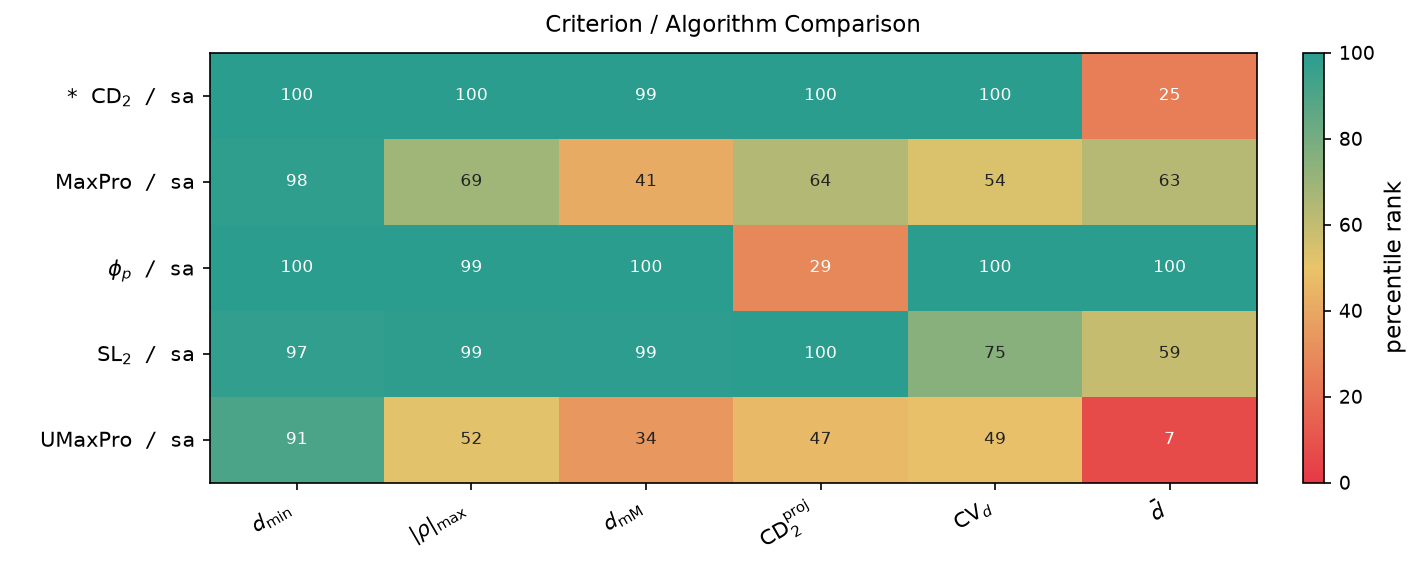
comparison.plot()(saved ascomparison_matrix_1.png): the percentile-rank heat map itself, one row per criterion and algorithm combination with the winning row starred; this is the comparison at a glance.comparison_table.md(saved to disk): columns are percentile ranks against a single shared Monte Carlo baseline, not raw criterion scores. Raw scores from different criteria are not comparable on their own scale, so ranking by percentile is the only sound way to put them side by side. The winning row is flagged.min_distance and max_abs_correlation are the two priority metrics here: a GP surrogate’s prediction variance grows where design points are far apart (min_distance), and correlated inputs make the individual effect of each factor harder to separate (max_abs_correlation). They are treated as competing objectives, not as a strict first/second order: the winner is the design closest to the ideal on both (see the Pareto/Utopia note below), so a design is never picked that sacrifices one badly for a marginal gain on the other.
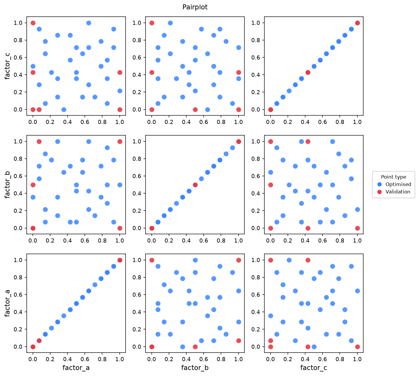
The winning design’s saved pairplot: an even spread in every panel is the visual signature of a good space-filling design.
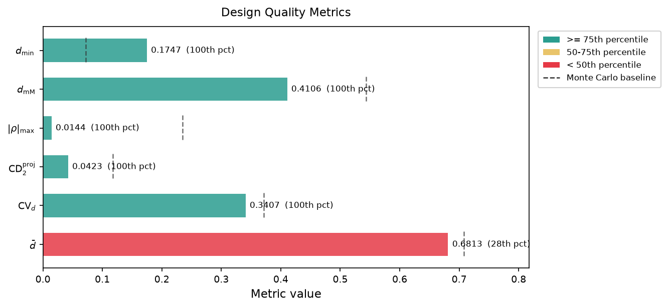
The saved quality plot: each metric’s percentile against the Monte Carlo baseline shown as a bar, so the winner’s quality is legible at a glance rather than read off a table.
winner_design.csv: the winning benchmark rows, ready for the downstream modelling step.
Mergen features used#
Sampler.compare(criteria=None, ...): criteria=None resolves to every criterion compatible with the space; since this space has no nominal factor, the QQ-family criteria are automatically excluded. Each combination is optimised n_repeats times (default 5) from independent, reproducible seeds, and ranked on the mean metric percentile so the choice does not hinge on a single lucky seed. The winner is chosen by a Pareto/Utopia rule over the priority metrics.ComparisonResult: .table, .best, .best_result.
comparison.table saved to outputs/comparison_table.md; the winning design saved as a pairplot (PNG) and a CSV.
quality_report()stays in the terminal.
Estimated runtime: a few minutes on one core (five criteria x five
repeats). On a multi-core machine, pass n_jobs=-1 (or a small number
like n_jobs=4) to compare() to run the repeats in parallel; the result
is identical, only faster. Leave n_jobs at its default to stay on a
single core.
from mergen import ParameterSpace, Sampler

# 1. Define a purely numeric parameter space.
space = ParameterSpace({
    'factor_a': ('continuous', 0.0, 1.0, {'resolution': 15, 'round': 3}),
    'factor_b': ('continuous', 0.0, 1.0, {'resolution': 15, 'round': 3}),
    'factor_c': ('continuous', 0.0, 1.0, {'resolution': 15, 'round': 3}),
})

# 2. Configure the sampler and compare every compatible criterion.
#    Each criterion/algorithm combination is optimised several times
#    (n_repeats default 5) and ranked on the mean metric percentile, so
#    the winner reflects typical rather than single-run performance. On
#    a multi-core machine add n_jobs=-1 to parallelise; the result is
#    unchanged.
sampler = Sampler(space)
sampler.set_design(n_samples=30)
comparison = sampler.compare(
    priority=('min_distance', 'max_abs_correlation'),
    n_jobs=1,  # one core; set n_jobs=-1 to use all cores (same result)
)

# 3. Save the comparison table itself: which criterion won, and by
#    how much on each quality metric. to_markdown() writes under the
#    output directory, creating it if needed.
comparison.to_markdown('comparison_table.md')
comparison.plot(save=True)

# 4. Inspect and save the winning design.
best = comparison.best_result
best.quality_report()
best.plot('pairplot', save=True)
best.plot('quality', save=True)
best.to_csv('winner_design.csv')
  [COMPARE]  cd2 + sa (5 repeats) ...
  [COMPARE]  maxpro + sa (5 repeats) ...
  [COMPARE]  phi_p + sa (5 repeats) ...
  [COMPARE]  stratified + sa (5 repeats) ...
  [COMPARE]  umaxpro + sa (5 repeats) ...
  [COMPARE]  Monte Carlo baseline (300 random designs, n=30) ...

════════════════════════════════════════════════════════════
  MERGEN — Space-filling Design
════════════════════════════════════════════════════════════
  Parameters      : 3
  Candidates      : 3,375
  n_samples       : 30  (prescribed_in=0, focus_in=0, optimised_slots=30)
  Total design    : 30
  Validation      : 6
  Criterion       : cd2
  Algorithm(s)    : sa
────────────────────────────────────────────────────────────

────────────────────────────────────────────────────────────
  MERGEN — Final Design
────────────────────────────────────────────────────────────
  Prescribed (in)  : 0
  Prescribed (out) : 0
  Focus (in)       : 0
  Focus (out)      : 0
  Optimised        : 30
  Total design     : 30
  Validation       : 6
════════════════════════════════════════════════════════════

════════════════════════════════════════════════════════════════════════
  MERGEN — Criterion / Algorithm Comparison
════════════════════════════════════════════════════════════════════════
  Priority: min_distance > max_abs_correlation   (percentile vs shared MC baseline, higher is better)
────────────────────────────────────────────────────────────────────────
best  criterion algorithm  min_distance  max_abs_correlation  minimax  projection_cd2  cv_distances  mean_distance
   *        cd2        sa         100.0                100.0     99.3           100.0         100.0           25.3
         maxpro        sa          98.3                 69.0     41.3            64.0          53.7           63.3
          phi_p        sa         100.0                 99.3    100.0            28.7         100.0          100.0
     stratified        sa          97.3                 98.7     99.0           100.0          75.0           59.0
        umaxpro        sa          91.0                 51.7     34.3            46.7          48.7            7.0
────────────────────────────────────────────────────────────────────────
  Best: criteria='cd2', algorithm='sa'
════════════════════════════════════════════════════════════════════════
  Saved: outputs/comparison_table.md
  Saved: outputs/comparison_matrix_1.png
  [METRICS]  Computing MC baseline (300 designs)...
  [METRICS]  MC baseline complete (300 designs).

════════════════════════════════════════════════════════════════════════
  MERGEN Design Metrics  (n=30, d=3)
════════════════════════════════════════════════════════════════════════
  Metric                      Value    Baseline  Better when        Rank
────────────────────────────────────────────────────────────────────────
  Min distance               0.1747      0.0720  higher        100th pct
  Minimax distance           0.4106      0.5394  lower          99th pct  *
  Max |correlation|          0.0144      0.2321  lower         100th pct
  2D projection CD2          0.0423      0.1187  lower         100th pct  *
  CV distances               0.3407      0.3711  lower         100th pct  *
  Mean distance              0.6813      0.7094  higher         25th pct
────────────────────────────────────────────────────────────────────────
  Criterion scores
────────────────────────────────────────────────────────────────────────
  CD2                            0.0575      0.1573  100th pct  lower
────────────────────────────────────────────────────────────────────────
  * = primarily optimised by 'cd2'
  For other priorities, see: mergen.criteria.list_criteria()
────────────────────────────────────────────────────────────────────────
  Baseline: 300 MC designs from feasible space  |  Rank = percentile among baseline designs
════════════════════════════════════════════════════════════════════════

  Saved: outputs/pairplot_4.png
  Saved: outputs/quality_1.png
  Saved: outputs/winner_design.csv  (36 rows)
Total running time of the script: (7 minutes 5.219 seconds)