

Note
Go to the end to download the full example code.
14_bsm_2hdm_phenomenology.py#
A Type-II Two-Higgs-Doublet-Model (2HDM) phenomenology study needs a set of benchmark points spread across the five free parameters of the model. Each benchmark will later be handed to downstream tools (for example 2HDMC, SuperIso, HiggsBounds/HiggsSignals) that compute flavour and collider observables and set limits. Mergen’s role is only to decide where in the five-dimensional parameter space the benchmarks should sit so the volume is covered efficiently with few points; it does not compute any cross-section, observable or limit — that is the downstream tool’s job.
This is where a space-filling design earns its keep. A naive grid at five levels per axis is 5**5 = 3125 points; a space-filling design covers the same volume with a few dozen well-separated benchmarks. A low-dimensional model (say a single VLQ with two free parameters) would not show this advantage — the method matters precisely because the 2HDM parameter space is five-dimensional.
Parameters#
Stepped grids, as real scans are stepped rather than continuous, with LaTeX names so the physics notation appears on the axes and in the exported header.
tan(beta): a log-like ladder [1, 2, 5, 10, 15, 20].
cos(beta - alpha): the alignment region, in steps around zero.
m_H (heavy CP-even scalar): 300-1500 GeV in 200 GeV steps.
m_A (CP-odd scalar): 300-1500 GeV in 200 GeV steps.
m_H+- (charged scalar): 300-1500 GeV in 200 GeV steps.
What to look at#
comparison_table.md (saved): all numeric criteria ranked by percentile against a shared Monte Carlo baseline. The question “did we cover the 5D space well?” maps directly to the min_distance and max_abs_correlation percentiles.
best_result.quality_report() (printed): the winning design’s coverage quality in five dimensions.
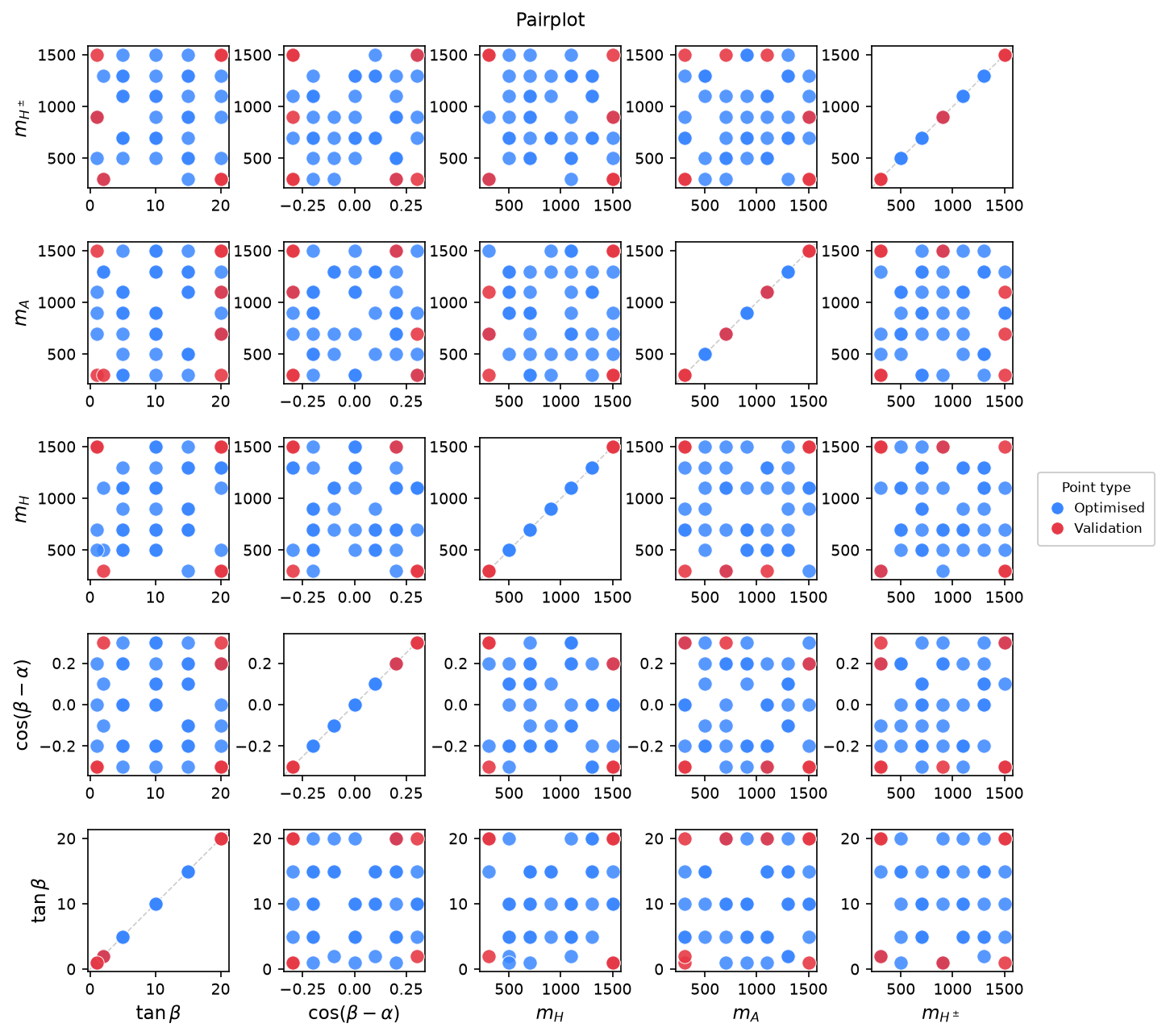
The saved 5x5 pairplot: even coverage across every pair of parameters is the visual sign that the benchmarks span the space rather than clustering.
benchmarks.csv: one row per benchmark point, with the LaTeX parameter names as headers, ready to feed the downstream chain.
Mergen features used#
LaTeX parameter names used directly as space keys, so they appear on plot axes and in the CSV header.
Sampler.compare(): all factors are numeric, so criteria=None sweeps the numeric criteria and ranks them on coverage percentiles. Each combination is optimised n_repeats times (default 5) from reproducible seeds and ranked on the mean metric percentile via a Pareto/Utopia rule, so the choice is stable rather than tied to one seed.
ComparisonResult.best_result and its saved ranking table.
Estimated runtime: several minutes on one core (several criteria in five dimensions, each repeated). On a multi-core machine pass n_jobs=-1 to compare() to parallelise the repeats (identical result, faster); leave it at the default to stay single-core.
from mergen import ParameterSpace, Sampler

# 1. Define the 2HDM parameter space on stepped grids. LaTeX names are
#    used verbatim as keys so the physics notation propagates to the
#    plot axes and the exported header.
space = ParameterSpace({
    r'$\tan\beta$':          [1, 2, 5, 10, 15, 20],
    r'$\cos(\beta-\alpha)$': [-0.3, -0.2, -0.1, 0.0, 0.1, 0.2, 0.3],
    r'$m_H$':                range(300, 1501, 200),
    r'$m_A$':                range(300, 1501, 200),
    r'$m_{H^\pm}$':          range(300, 1501, 200),
})

# 2. Compare the numeric criteria and pick the best coverage. The
#    optimiser is tuned down so the five-dimensional sweep is quick for
#    a demonstration.
sampler = Sampler(space)
sampler.set_design(n_samples=40)
sampler.set_optimizer('sa', n_restarts=2, max_iter=400)
comparison = sampler.compare(
    n_jobs=1,  # one core; set n_jobs=-1 to use all cores (same result)
)

# 3. Save the ranking table.
comparison.to_markdown('comparison_table.md')

# 4. Inspect and save the winning set of benchmark points.
best = comparison.best_result
best.quality_report()
best.plot('pairplot', save=True)
best.to_csv('benchmarks.csv')
  [COMPARE]  cd2 + sa (5 repeats) ...
  [COMPARE]  maxpro + sa (5 repeats) ...
  [COMPARE]  phi_p + sa (5 repeats) ...
  [COMPARE]  stratified + sa (5 repeats) ...
  [COMPARE]  umaxpro + sa (5 repeats) ...
  [COMPARE]  Monte Carlo baseline (300 random designs, n=40) ...
  [WARNING]  n_samples (40) < recommended 10*n_parameters (50, Loeppky et al. 2009). Design quality may be reduced.

════════════════════════════════════════════════════════════
  MERGEN — Space-filling Design
════════════════════════════════════════════════════════════
  Parameters      : 5
  Candidates      : 14,406
  n_samples       : 40  (prescribed_in=0, focus_in=0, optimised_slots=40)
  Total design    : 40
  Validation      : 8
  Criterion       : cd2
  Algorithm(s)    : sa
────────────────────────────────────────────────────────────

────────────────────────────────────────────────────────────
  MERGEN — Final Design
────────────────────────────────────────────────────────────
  Prescribed (in)  : 0
  Prescribed (out) : 0
  Focus (in)       : 0
  Focus (out)      : 0
  Optimised        : 40
  Total design     : 40
  Validation       : 8
════════════════════════════════════════════════════════════

════════════════════════════════════════════════════════════════════════
  MERGEN — Criterion / Algorithm Comparison
════════════════════════════════════════════════════════════════════════
  Priority: min_distance > max_abs_correlation   (percentile vs shared MC baseline, higher is better)
────────────────────────────────────────────────────────────────────────
best  criterion algorithm  min_distance  max_abs_correlation  minimax  projection_cd2  cv_distances  mean_distance
   *        cd2        sa          94.3                100.0     97.7           100.0          99.7            0.3
         maxpro        sa          99.8                 60.3     54.5            24.7          90.7           96.0
          phi_p        sa         100.0                 92.0     98.0            24.7         100.0          100.0
     stratified        sa          94.3                100.0     99.0            96.3          90.7           75.7
        umaxpro        sa          88.8                 58.0     54.5            24.7          22.7           48.7
────────────────────────────────────────────────────────────────────────
  Best: criteria='cd2', algorithm='sa'
════════════════════════════════════════════════════════════════════════
  Saved: outputs/comparison_table.md
  [METRICS]  Computing MC baseline (300 designs)...
  [METRICS]  MC baseline complete (300 designs).

════════════════════════════════════════════════════════════════════════
  MERGEN Design Metrics  (n=40, d=5)
════════════════════════════════════════════════════════════════════════
  Metric                      Value    Baseline  Better when        Rank
────────────────────────────────────────────────────────────────────────
  Min distance               0.2887      0.2357  higher         94th pct
  Minimax distance           0.8087      0.9051  lower          98th pct  *
  Max |correlation|          0.0786      0.2955  lower         100th pct
  2D projection CD2          0.0862      0.1576  lower         100th pct  *
  CV distances               0.2559      0.2790  lower         100th pct  *
  Mean distance              0.9347      1.0360  higher          0th pct
────────────────────────────────────────────────────────────────────────
  Criterion scores
────────────────────────────────────────────────────────────────────────
  CD2                            0.1660      0.3147  100th pct  lower
────────────────────────────────────────────────────────────────────────
  * = primarily optimised by 'cd2'
  For other priorities, see: mergen.criteria.list_criteria()
────────────────────────────────────────────────────────────────────────
  Baseline: 300 MC designs from feasible space  |  Rank = percentile among baseline designs
════════════════════════════════════════════════════════════════════════

  Saved: outputs/pairplot_16.png
  Saved: outputs/benchmarks.csv  (48 rows)
Total running time of the script: (1 minutes 2.839 seconds)